Microsoft Azure Machine Learning Studio is an easy drag and drop cloud tool that enables you to perform machine learning at scale. It allows you to upload your own custom data-set and perform supervised or unsupervised machine learning tasks on it.
To access this Microsoft Azure Machine Learning Studio just log into Azure account. If you don’t have one, then you can create here. One good initial feature about Microsoft Azure is that it offers $200 free credits on every new account without providing any credit card details.
Here is a brief video explaining about how to use Microsoft Azure Machine Learning Studio.
In this blog, we shall learn how to perform Linear Regression on House Price Prediction Dataset using Microsoft Azure Machine Learning Studio.
TABLE OF CONTENTS
- Exploring Microsoft Azure Machine Learning Studio
- Creating a New Experiment and Loading Custom Dataset
- Visualizing and Analyzing the data-set
- Pre-processing the data-set
- Using a machine learning model to train the dataset
- Scoring the dataset
- Performing Cross-Validation
- Evaluating the results
- Deploying it as a web-service
- Summary
Exploring Microsoft Azure Machine Learning Studio
Microsoft Azure Machine Learning Studio is a powerful software tool that helps you to process your data using inbuilt modules without writing any code. But, along with this it also allows the users to write custom R and python script for performing some advance processing on the data.
Microsoft Azure Machine Learning Studio has a well-designed user-interface. Once you login into your workspace, look at the left panel. This left panel has following options:
- PROJECT : Shows a list of Projects you created in this studio. Each project can have different assets. Assets comprises of experiments, web-services, notebooks, datasets, and trained-model.
- EXPERIMENTS : Shows a list of experiments you created in this studio. AMLS provides sample experiments which guides how to do machine learning using this studio. After clicking experiments, click the SAMPLE tab to view the sample experiments.
- WEB SERVICES : You can deploy the experiment as either a Classic web service, or as a New web service that’s based on Azure Resource Manager. This article shows how to deploy your experiment as a web service.
- NOTEBOOKS : You can create new Jupyter Notebook here in studio hosted on Azure cloud. This notebook will open in a new tab and you can use it for quickly running code, visualizing data, exploring insights, and trying out ideas. You can learn more about this here.
- DATASETS : Here, you can find all your uploaded datasets. You can upload datasets from your local file in this studio. Microsoft Azure Machine Learning Studio gives you about 10 GB of storage for this.
- TRAINED MODELS : Once you convert your training experiment to a predictive experiment, azure automatically store it as a trained mode. Trained model is required for ‘Setting up a Web-Service’.
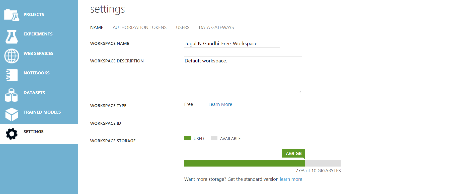
- SETTINGS : You can view your account setting over here. The most useful thing to see over it is how much workspace storage has been used.
Creating a New Experiment and Loading Custom Dataset
In this exercise, we are going to load a public data-set hosted by kaggle. You can find and download this data-set here. Download it and store it on your local drive. This dataset contains house sale prices for King County. This data-set consists of 21 columns and 21613 rows. Out of these 21 columns, the ‘price’ column is called label(one which we are trying to predict), and the remaining 20 columns are called as features(independent predictors). Each row in dataset is called as observation or data-point. Once logged in Azure Machine Learning Studio, perform the following steps:
-
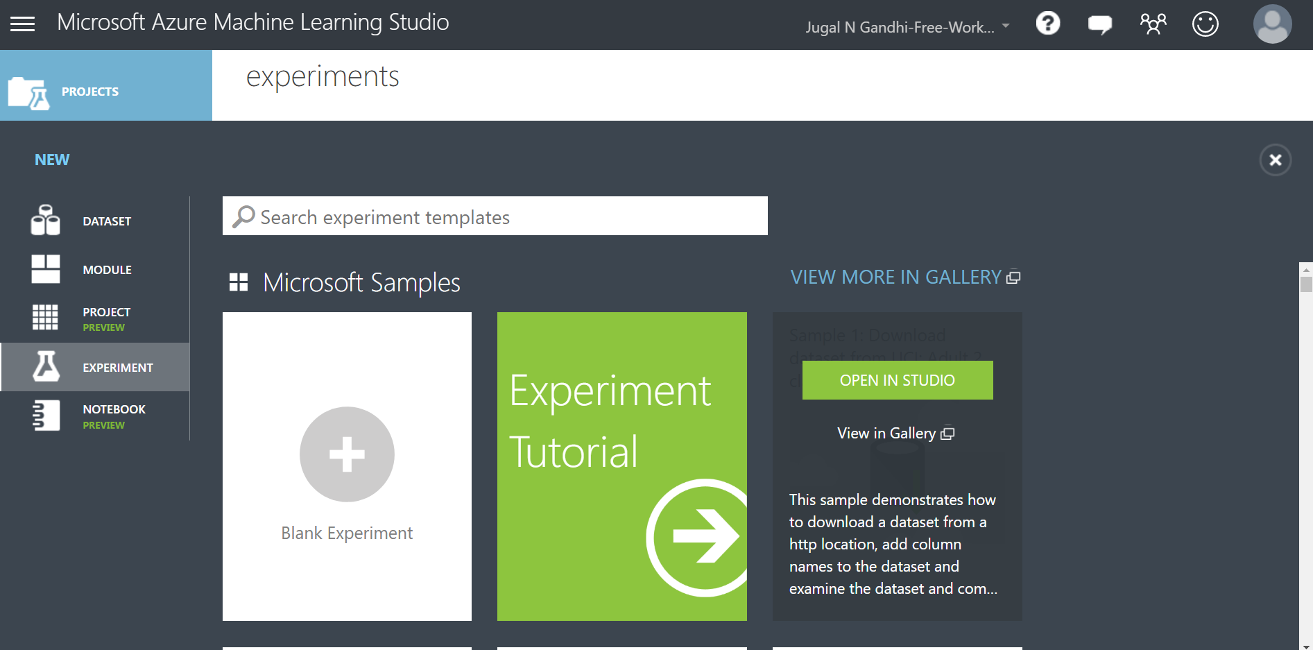
STEP 1: Create a new experiment by pressing +NEW at the bottom left corner and selecting Blank Experiment.
-
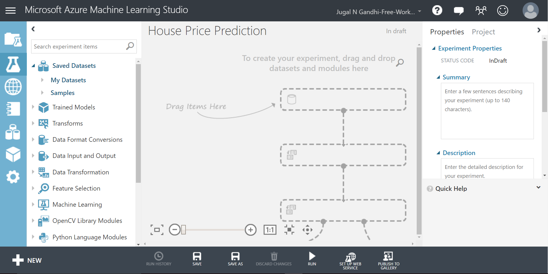
STEP 2: Change the default name of experiment at the top left corner to “House Price Prediction”.
-
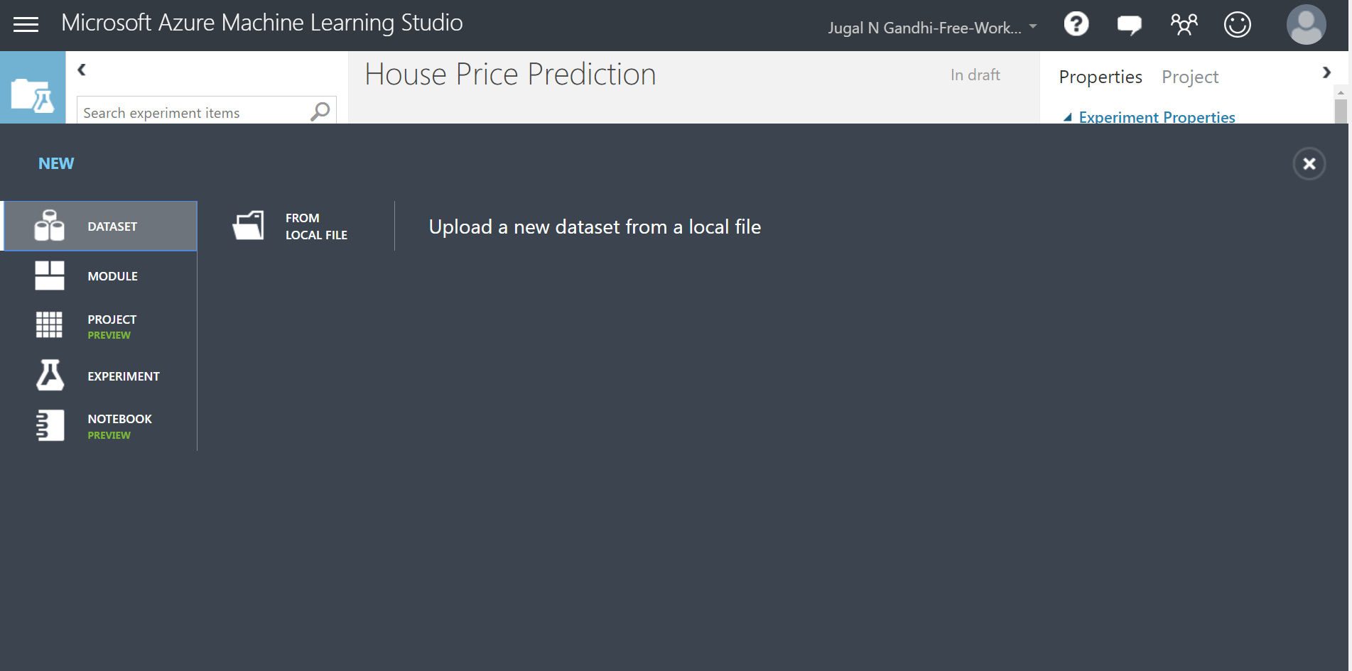
STEP 3: Upload your downloaded data-set from your local drive by clicking +NEW and having selected DATASET select FROM LOCAL FILE. Give it a proper name and you can find your custom data-set under Saved Datasets option present in the left modules palette. In my case I have named this data-set as “kc_house_data.csv”.
-
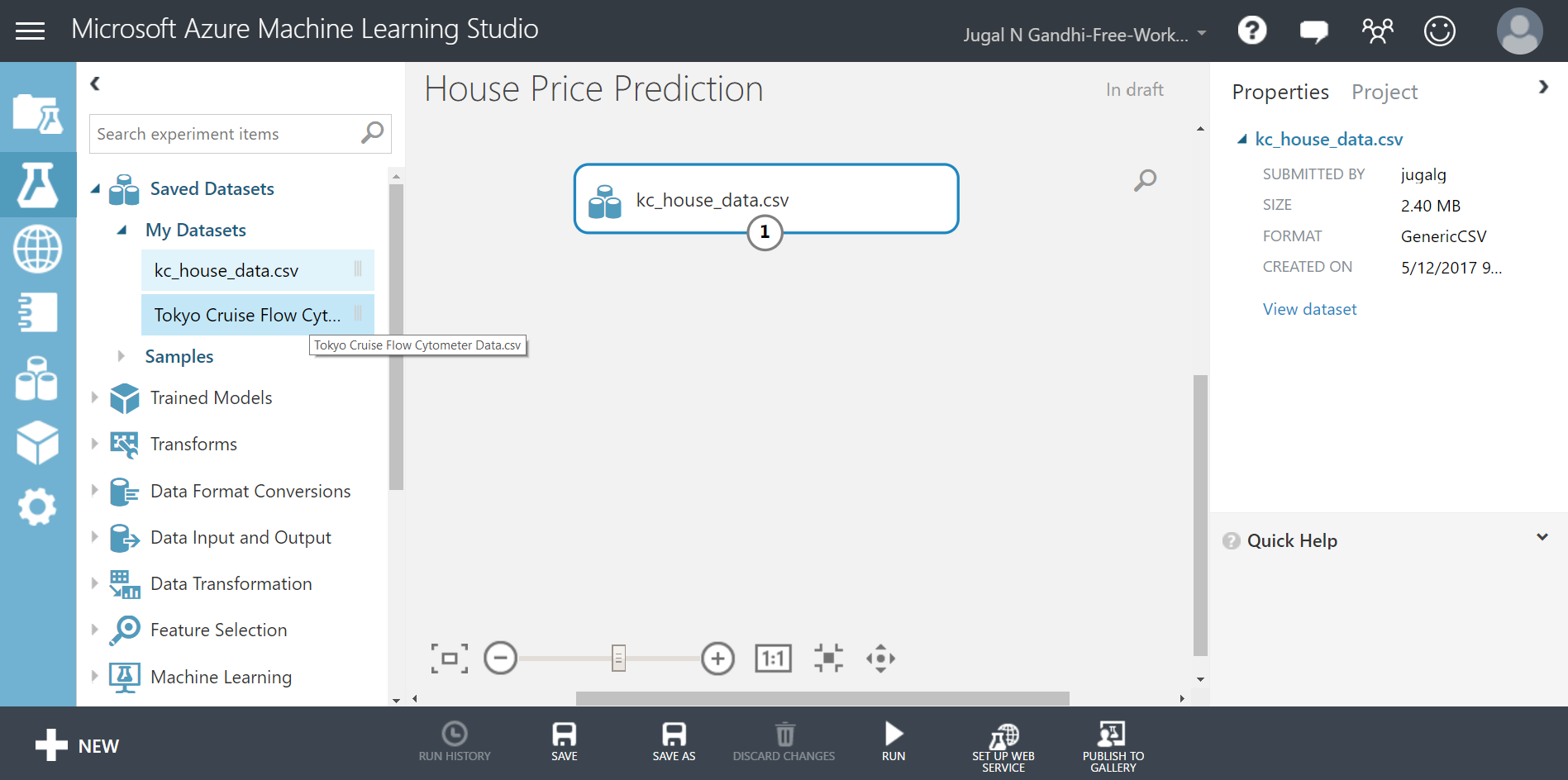
STEP 4: Select your uploaded data-set in Saved Datasets option present in the left modules palette of your experiment. Now drag and drop it under your experiment canvas.
Visualizing and Analyzing the data-set
Here, our custom data-set is about predicting the prices of ghouses. There are two types of machine learning problems: one is supervised learning problems and other is unsupervised machine learning. Here, the house price prediction problem is a supervised machine learning problem (classification problem and to be precise a regression problem). Now that we have our custom data-set present in our experiment, the next things to do here is to visualize it, analyze it and pre-process it.
1. VISUALIZE
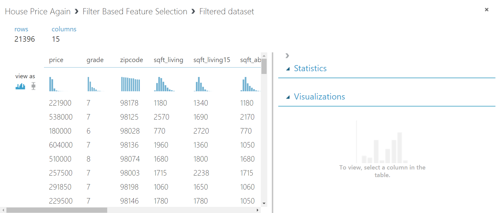
Microsoft Azure Machine Learning Studio provides you the option to visualize your data-set.
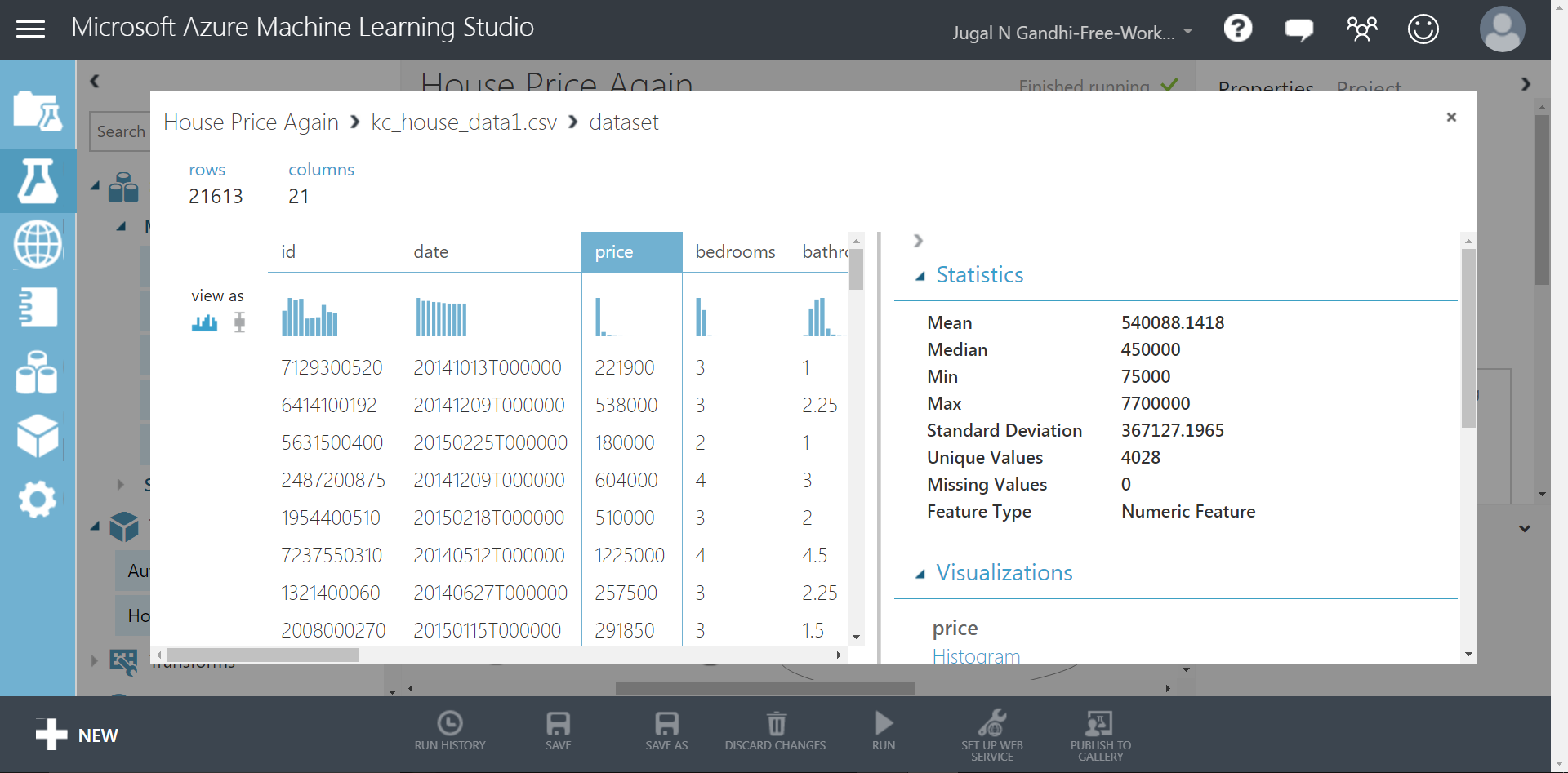
Microsoft Azure Machine Learning Studio only shows some 100 rows of your dataset, but not the complete dataset. Here, you can select any feature column and the side pane will show you statistics and histogram related to that feature column. This helps you to get meaningful insight of your dataset.
2. ANALYZE
When doing machine learning it is important to get insights of your dataset. Analzying here in our dataset, means to carefully look at the values of feature columns. There are two types of features in machine learning: numeric and non-numeric feature. Numeric features are further divided into two categories: catergorical numeric feature and continuous numerical feature. By default, Microsoft Azure Machine Learning Studio would tag each and every feature column as ‘numeric’(representing continuous numeric), if it has numbers in it. It is very important to analyze the type of feature and tag it with that appropriate type, because it affects the output of the machine learning model.
In the case of continuous features, there exist a measurable difference between possible feature values. For example: distance, time, cost, tempature, etc. With categorical features, there is a specified number of discrete, possible feature values. For example: Colors, Class, Car Model, etc.
After looking at the values of feature columns in dataset we realize that feature columns like ‘grade, waterfront, view, bedroom, condition and zipcode’ should actually be categorical features than the default continuous numeric feature. So, this needs to be changed.
Also, the feature column ‘yr_renovated’ is mostly filled with zeroes. Only few rows have non-zero values. Here, we can replace the entire column with only two values : 0(represting the house was never renovated) adn 1(representing the house was renovated).
All the analyzed points needs to be processed in ‘Pre-Process’ Task.
Pre-processing the data-set
The goal of preprocessing task is to make our data-set ready for training the machine learning model.
According to wikipedia, data pre-processing includes cleaning, instance selection, normalization, transformation, feature extraction and selection, etc. According to CCSU, tasks in data preprocessing are:
- Data Discretization
- Data Cleaning
- Data Transformation
- Data Reduction
1. Data Discretization
Data discretization is a part of data reduction, replacing numerical attributes with categorical(ordinal/nominal) ones. As discussed in the ‘Analyze’ section, there are some feature columns(grade, waterfornt, view, bedroom, condition and zipcode) whose data types need to be changed to catergorical. In MAMl, you can do this by doing following steps:
-
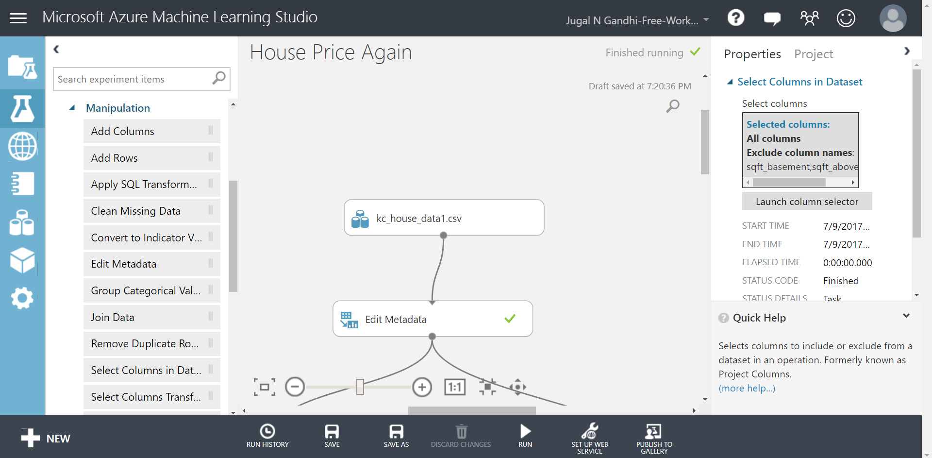
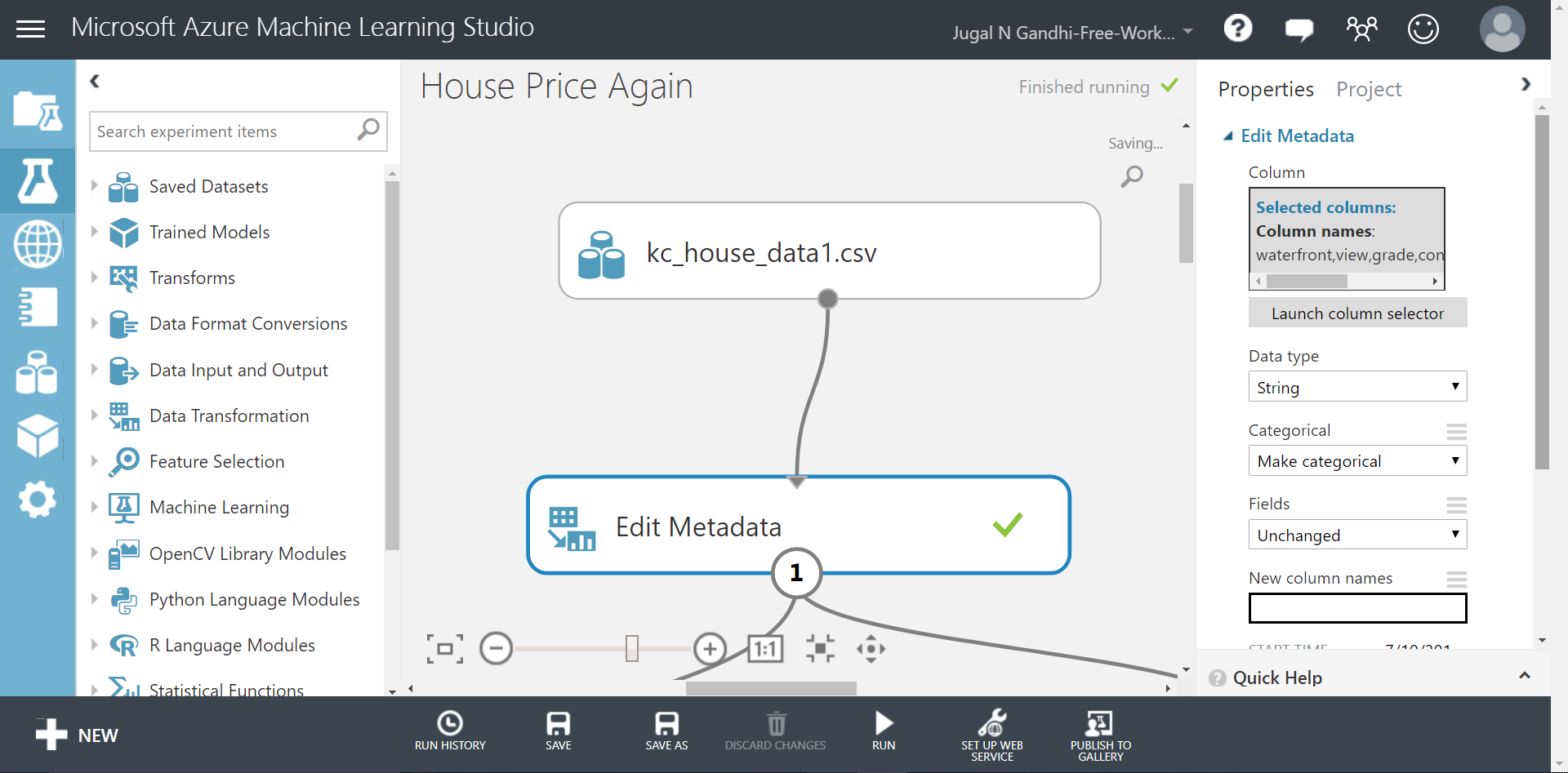
STEP 1: Drag the Edit Metadata module under your experiment canvas.
-
STEP 2: Connect the dataset to this Edit Metadata module.
-
STEP 3: Select the Edit Metadata module and edit the right panel to select all the columns you want to change to categorical type. Here we select ‘grade, waterfornt, view, bedroom, condition and zipcode’ feature columns. Under the Data type dropdown menu we select “String”(here String or Integer both works), and under the Categorical drop down menu we select “Make Categorical”.
-
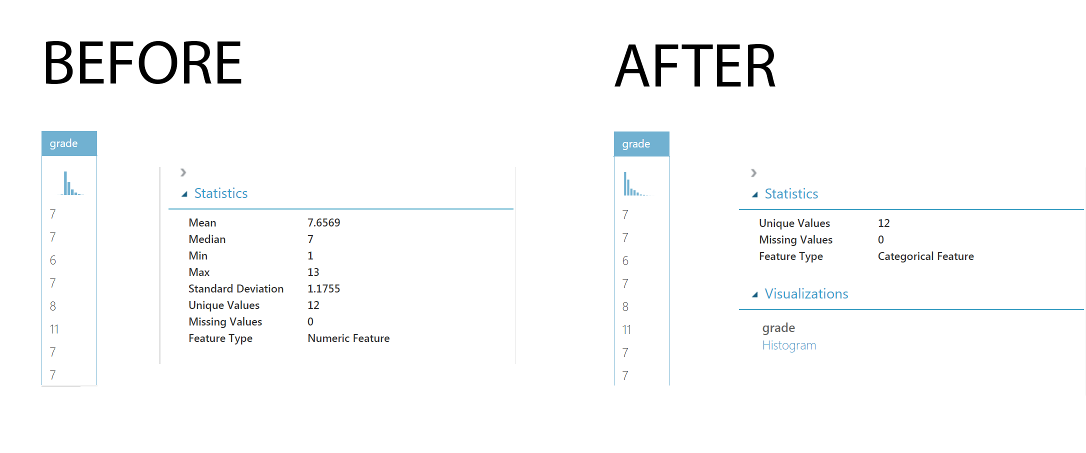
STEP 4: Run the experiment and right click the Edit Metadata module to verify the data-types of feature columns. This also changes the histogram and statistics values for the modified feature columns.
2. Data Cleaning
Data cleaning includes: fill in missing values, smooth noisy data, identify or remove outliers, and resolve inconsistencies. MAML provides different modules for cleaning up your dataset. Lets perform some of these steps:
i) Handling Missing Values: Find out missing values in feature columns and either Replace or Clip them. ‘Replace’ means replacing missing values by using many methods. One method is to replcae them with average value of that feature column. ‘Clip’ means to remove the entire row which has missing values in it.
Here, our dataset has no missing values.
ii) Identify or remove outliers: Here, when we visualize the ‘sqft_living’ column, then we see that peaks of this columns has some outliers. The goal here is to remove some rows from this column which has values greater than 99 percentile threshold. There is no simple way to do this in MAML. So to achieve this we have to perform following three steps:
-
STEP 1: Select Data Transformation -> Scale and Reduce option from left panel and drag the Clip Values module in your experiment canvas. Adjust the values in the right panel as shown in the figure below.
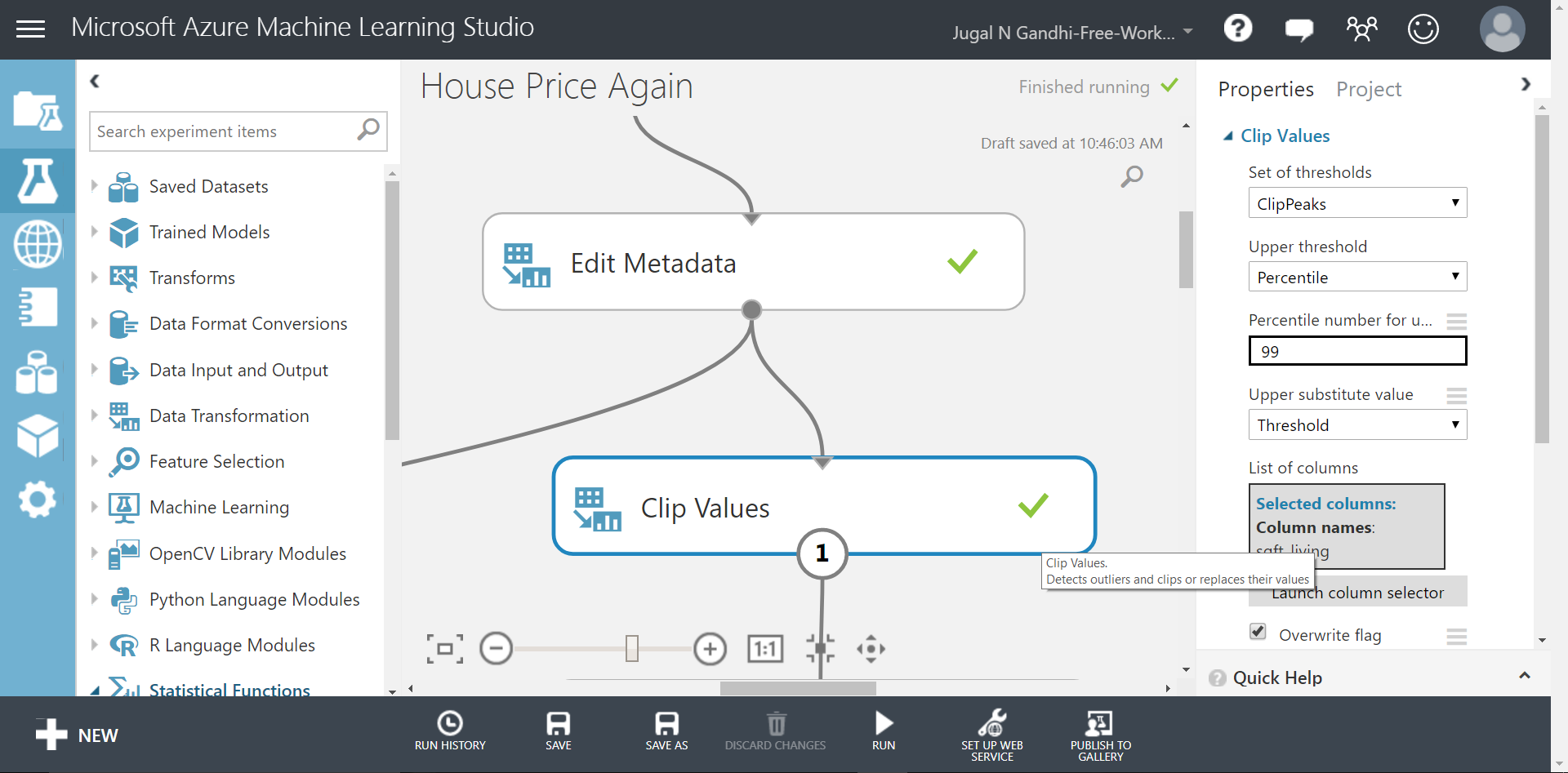
This shall add a new column in your dataset called ‘sqft_living_clipped’ with two values: False(Denoting the value is below the threshold) and True(Denoting the value is above the threshold).
-
STEP 2: Select Data Transformation -> Manipulation option from left panel and drag the Edit Metadata module in your experiment canvas. Adjust the values in the right panel as shown in the figure below.
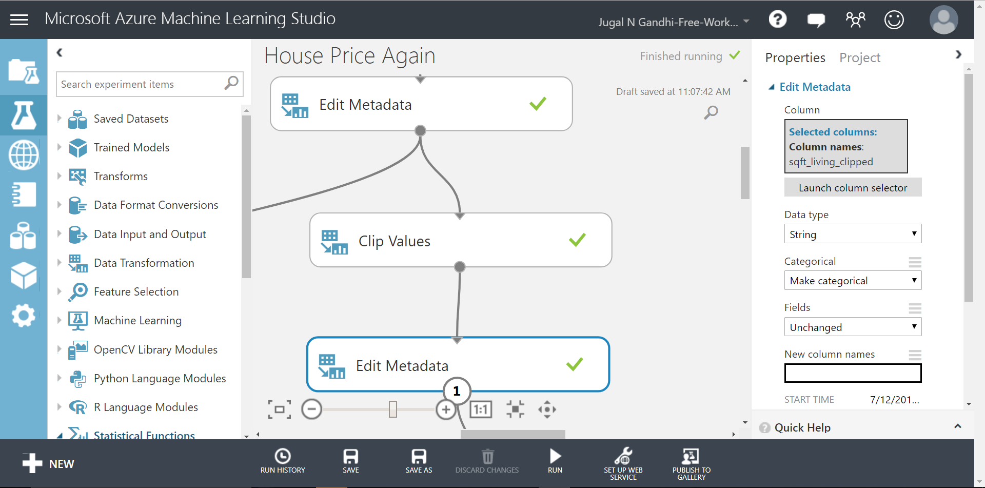
This will convert your ‘sqft_living_clipped’ column from ‘Boolean’ type to ‘String’ type so that you can query the column to remove some rows.
-
STEP 3: Select Data Transformation -> Sample and Split option from left panel and drag the Split Data module in your experiment canvas. Adjust the values in the right panel as shown in the figure below.
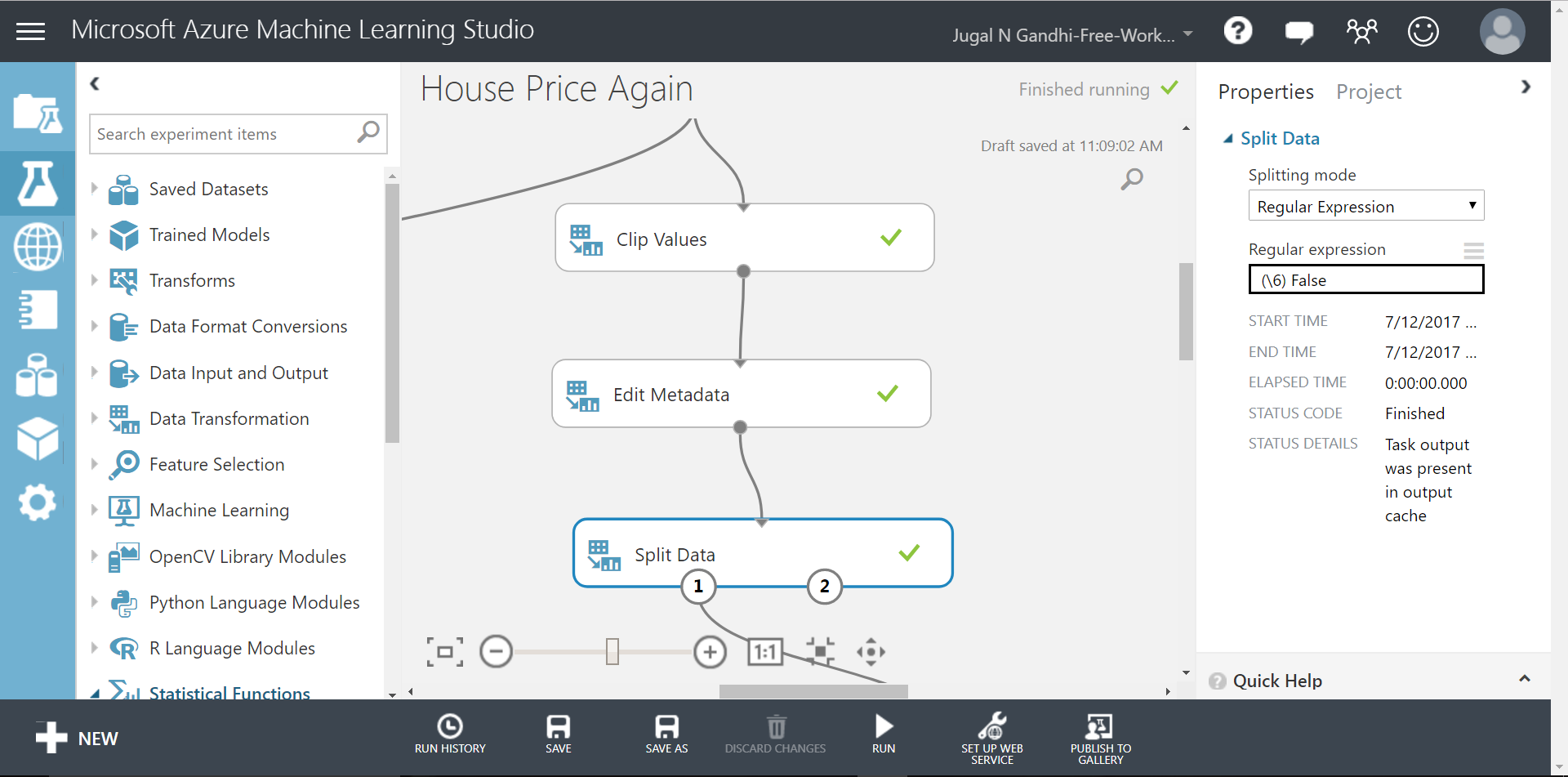
This will split your data according to the regular expression written. The regular expression above selects all rows from a column with index #2 that has value equal to ‘False’.
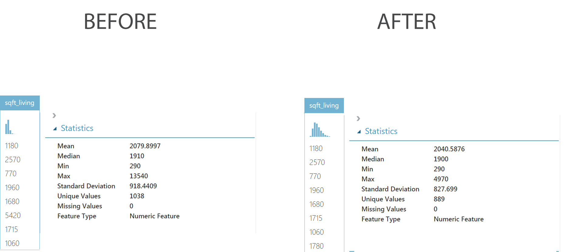
The result of these three steps is that we have removed outliers from ‘sqft_living’ column. This can be shown from the figure below. And now we have better normal distribution of data.
3. Data Transformation
Data Transformation includes normalization and aggregation. Normalization involves converting all of your columns values to same scale. This is done when there is significant difference between the ranges of your feature column values. The reason to do normalization is that you dont want one of your feature column values to dominate in the procedure of predicting target variable. Normalization essentially regularizes all of your feature columns.
It also includes adjustment of the column values. As discussed in “Analyze” section, we have to adjust the values of ‘yr_renowated’ feature column. To achieve these lets perform following steps:
-
STEP 1: Select Statistical Functions option from left panel and drag the Apply Math Operation module in your experiment canvas. Adjust the values in the right panel as shown in the figure below.
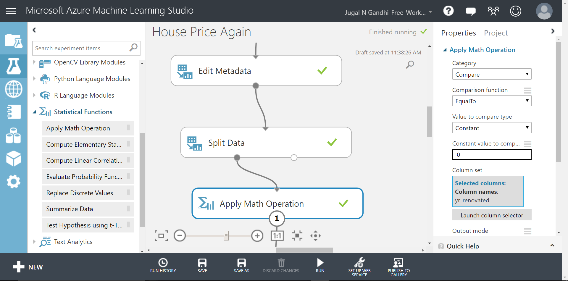
This module compares the selected feature column(in this case “yr_renowated” feature column), with a constant and replaces the feature column values with either: True(if the value matches the constant) or False(if the value doesn’t match the constant). Here, under Output Mode drop down menu we select Inplace option. This changes the selected feature column value in place.
-
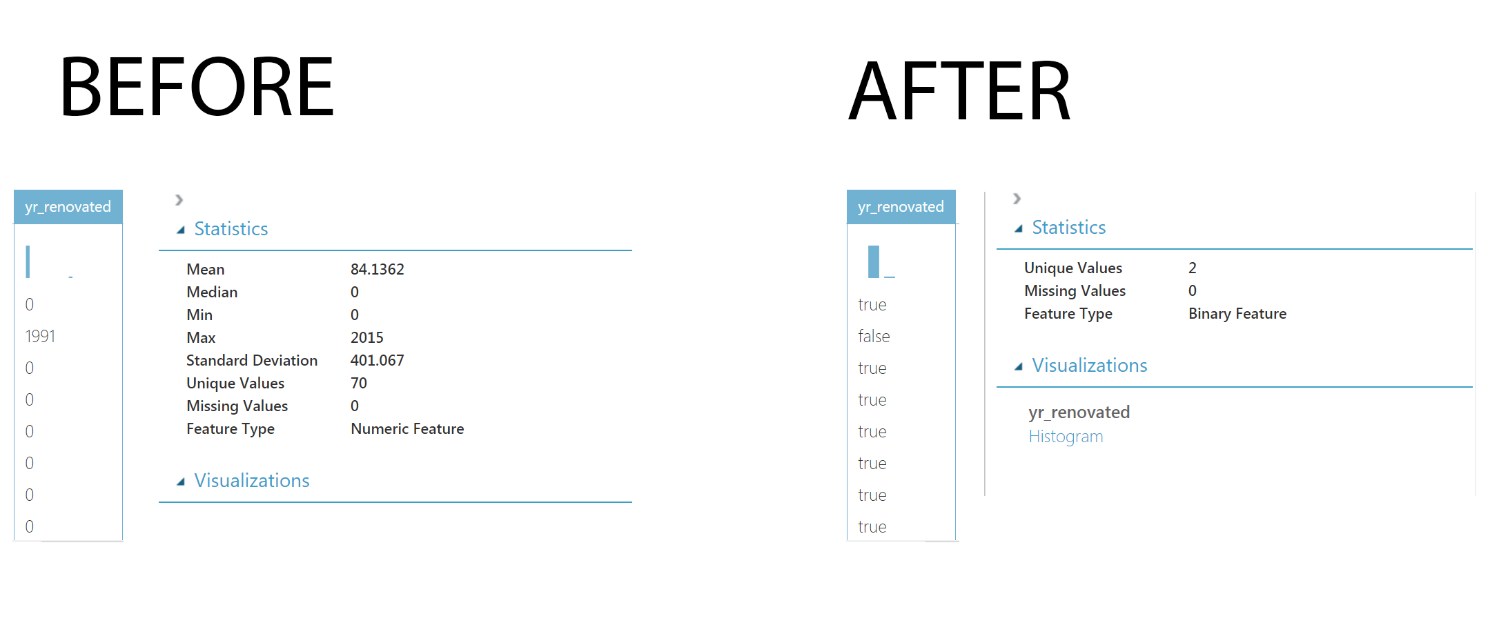
STEP 2: Run the experiment and right click the Apply Math Operation module to view the change in the ‘yr_renowated’ feature column. You can see that the data type of ‘yr_renowated’ feature column has now changed to ‘boolean’.
4. Data Reduction
Data reduction means reducing the volume but producing the same or similar analytical results. Data reduction is often termed as ‘Dimensionality Reduction’ in machine learning, where-in advanced techniques like “PCA” are used. Here, we shall reduce the data by removing unrelated and unnecessary data.
i) Removing unimportant feature columns: Some unuseful columns should be removed manually. These columns have no relation with the target label. Sometimes, this information can be obtained from domain expert who knows details about the meaning of the dataset. Here, in our case the unimportant feature columns are ‘sqft_living_clipped’ and ‘id’.
-
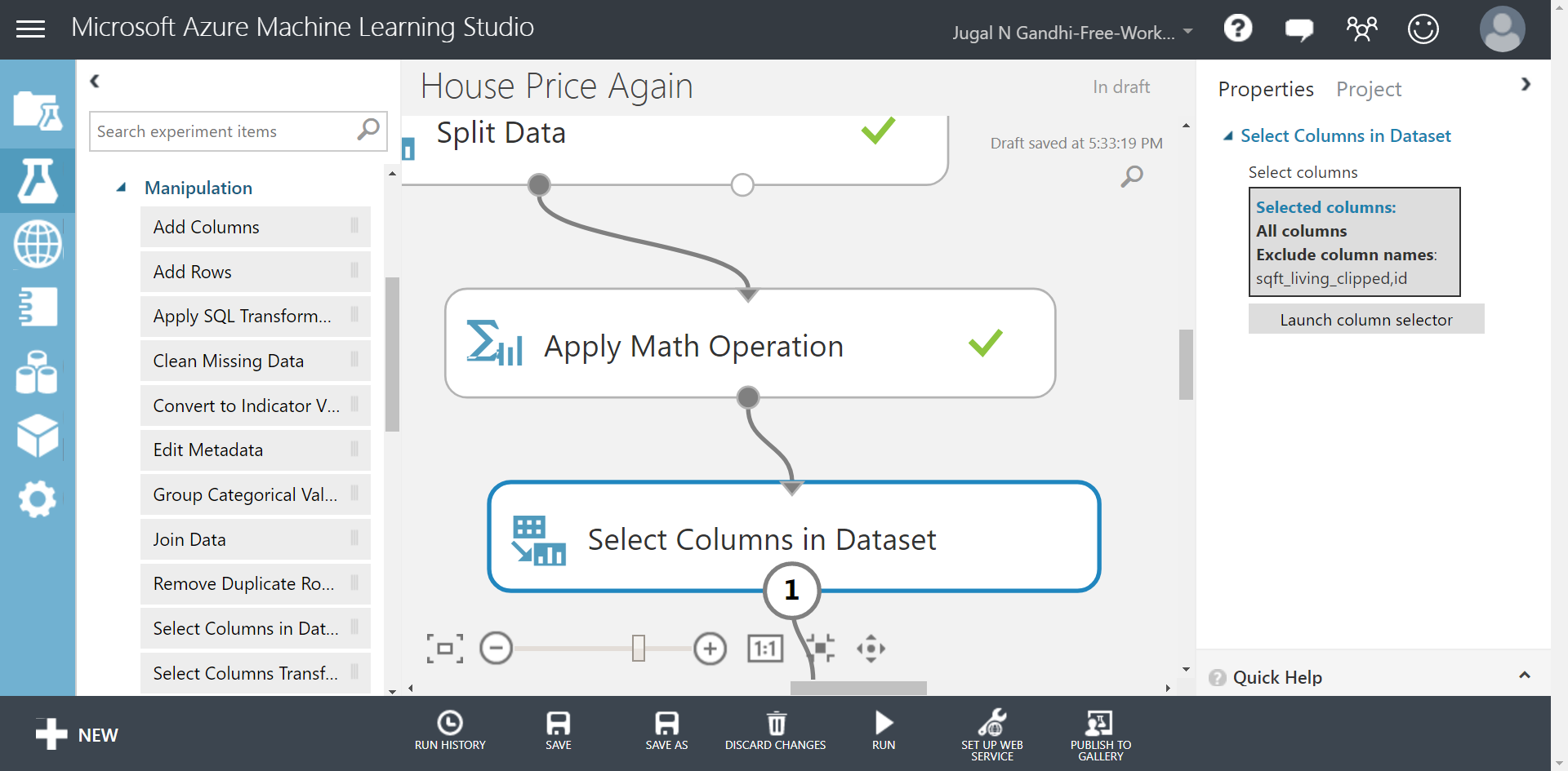
STEP 1: Select Data Transformation -> Manipulation option from left panel and drag the Select Columns in Dataset module in your experiment canvas. Then, select the Select Columns in Dataset module and in the right side panel click the Launch column selector to exclude two feature columns: ‘sqft_living_clipped’ and ‘id’.
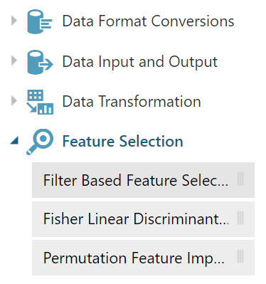
ii) Removing unrelated feature columns: Not all the feature columns are useful in predicting the target variable. Thus, we need to first find co-relation of the given features with the respective target column. Fortunately, MAML provides various modules under Feature Selection option. Out of three options available here we shall select Filter Based Feature Selection module.
-
STEP 1: Drag the Filter Based Feature Selection module under your experiment canvas. Connect this module.
-
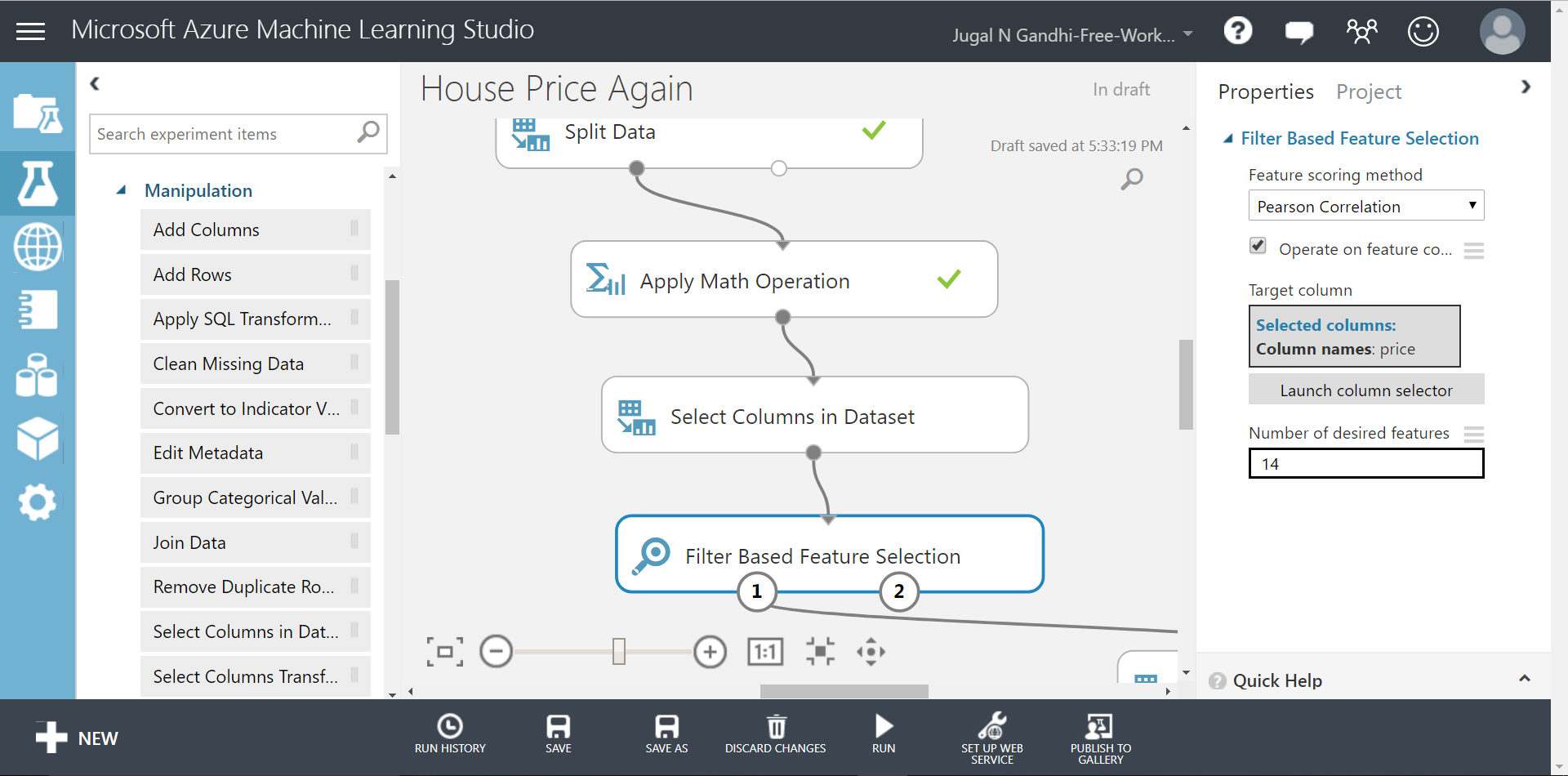
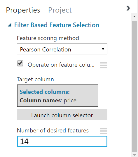
STEP 2: Select the Filter Based Feature Selection module and edit the right panel as shown below
-
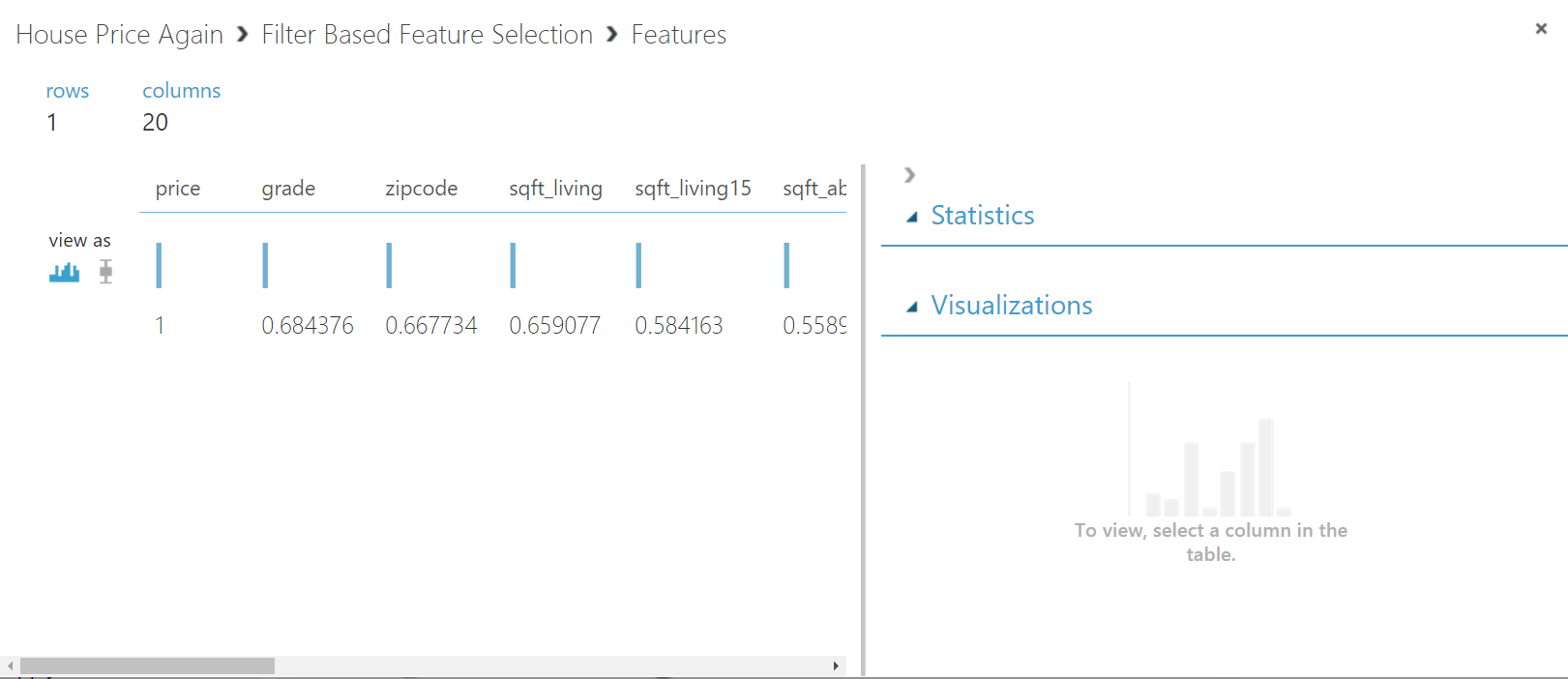
STEP 3: Run the experiment and right click the Filter Based Feature Selection to visualize the correlations of features with the target column. There are two circles attached with the Filter Based Feature Selection module. When you select the second circle it shows you the value of correlation of each column with the target column. The first circle output the 14 most correlated features of your dataset along with the target label column.
Also, clicking the second circle will show you the correlation values between the feature columns and target label.
Using a machine learning model to train the dataset
In this exercise we shall explore how to train a Linear Regression model in Microsoft Azure Machine Learning Studio.
-
STEP 1: Split your data-set into training part and test-part.
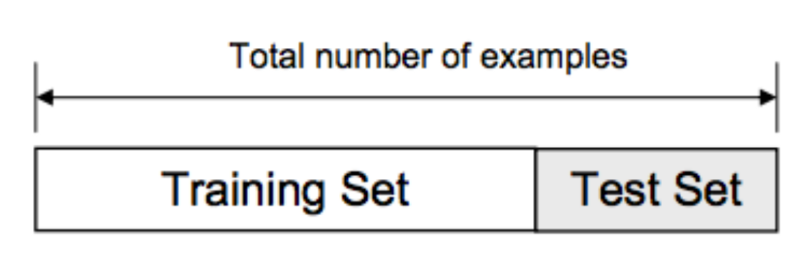
Usual thumb rule for a test-train split is to keep (1/3)rd part testing and (2/3)rd part for training. Though, you are free to choose the ratio of test-train split but always remember to have more training data then testing data. Here, we are going to use 70% of training examples for training.
Select Data Transformation -> Sample and Split option from left panel and drag the Split Data module in your experiment canvas. Adjust the values in the right panel as shown in the figure below.
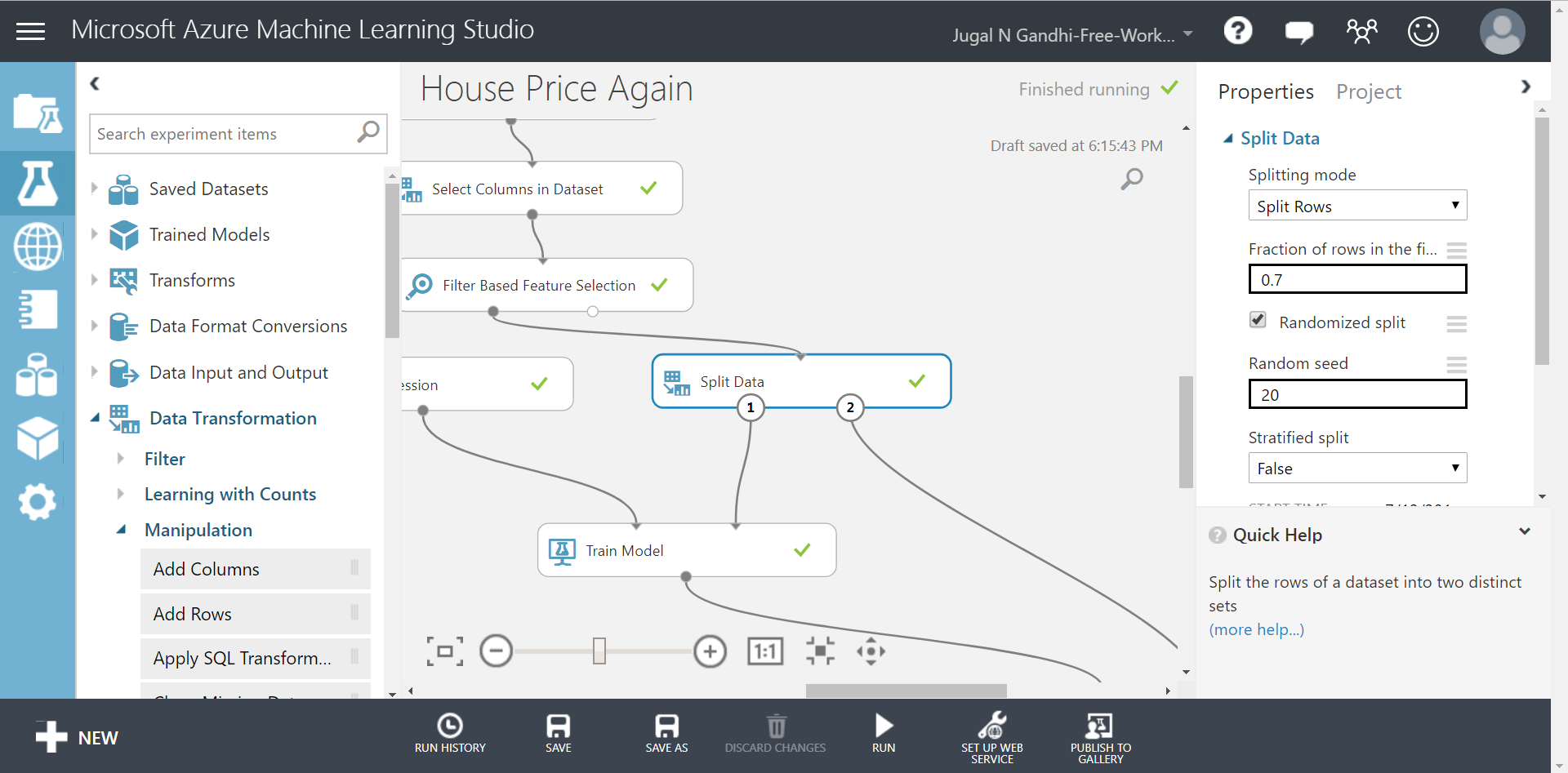
This shall split your data-set into training part(represented by circle #1) and test part(represented in circle #2). We will use the training data and send it to train a Linear Regression model.
-
STEP 2: Select your machine learning model.
Here, we know that we are dealing with a regression problem. So, lets select Machine Learning -> Initialize Model -> Regression and drag the Linear Regression module in your experiment canvas. Adjust the values in the right panel as shown in the figure below.
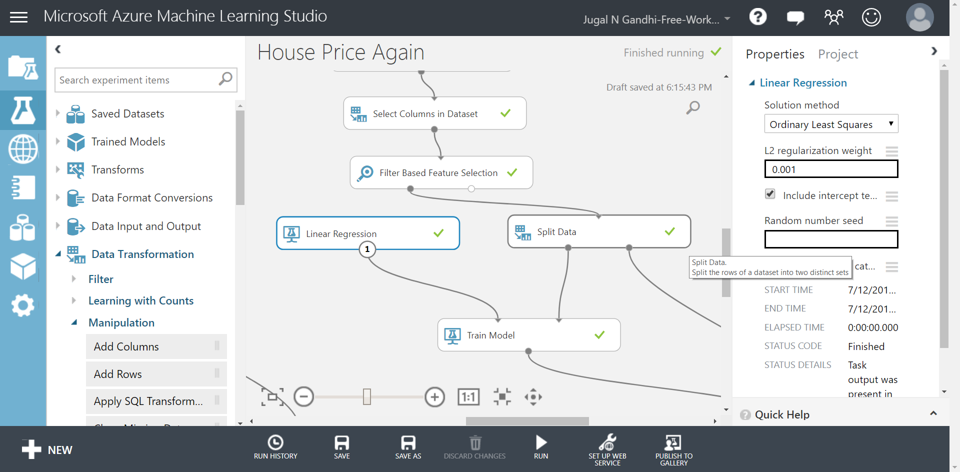
Our Linear Regression model is using Ordinary Least Squares method to project a line passing through all the data points present in training dataset. Ordinary Least Squares(OLS) method works by minimizing the sum of the squares of the differences between the observed datapoints and the predicted value.
-
STEP 3: Train your machine learning model.
Select Machine Learning -> Train and drag the Train Model module in your experiment canvas. In the right panel select price column which is our target column.
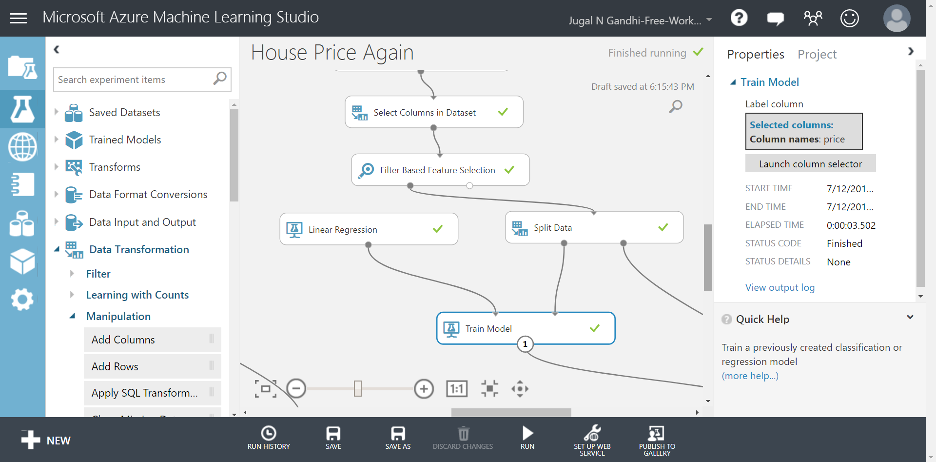
Connect the training part of your dataset and Linear Regression module to this Train Model module.
Scoring the dataset
In this exercise we shall learn how to score the test data-points after training machine learning model. Scoring the dataset means to take the test data and predict the target variable for this test data absed on the rules learnt from analyzing training data.
-
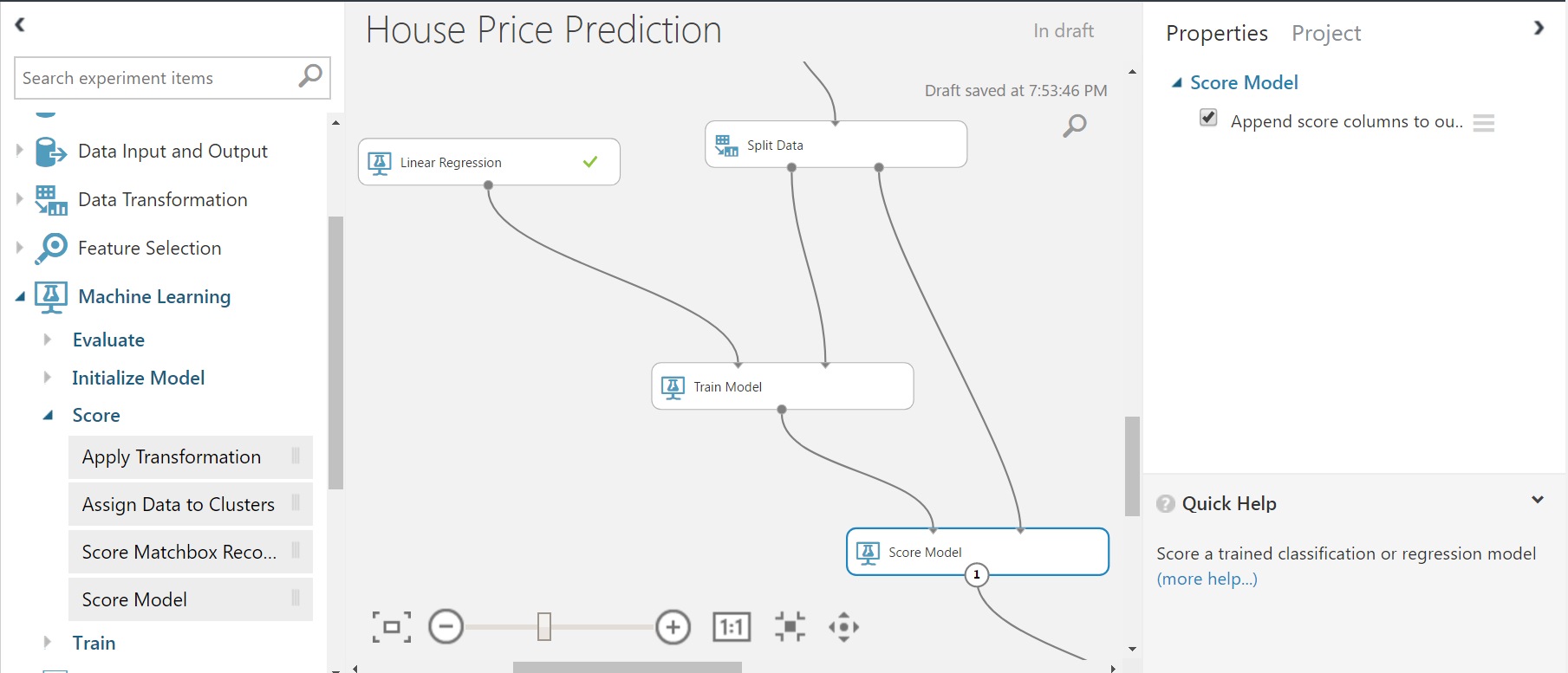
STEP 1: Select Machine Learning->Score from the left panel and drag the Score Model module in you experiment canvas.
-
STEP 2: Select the Score Model module and click to visualize the newly added Scored Labels column. As, shown in the figure below, we can see the differences between actual(‘Price’ feature column) and predicted(‘Scored Labels’ column).
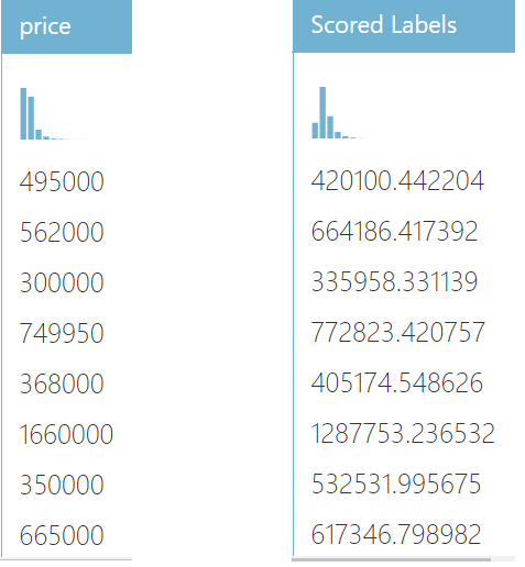
We can see here that predicted values are closer to the actual values. But just by looking we cannot compare and evaluate how well our linear regression model did. MAML provides modules for evaluating the machine learning models.
Performing Cross-Validation
As we saw above, we used top 70% of dataset to train and remaining bottom 30% for testing. This is one way of splitting. You can even take the bottom 70% of your dataset to train and the top 30% of your dataset to test. There are several such possible combinations. A good machine learning model should give you good accuracy on all such possible combinations. Cross Validation technique creates several such combinations and evaluates your model accuracy for all those combination. Cross-validation is an important technique used in machine learning to assess both the variability of a dataset and the reliability of any model trained using that data.
Cross-validation is an important technique used in machine learning to assess both the variability of a dataset and the reliability of any model trained using that data. Here, in MAML, Cross-Validate Model module defaults to 10 folds.
To perform cross validation of your dataset, do the following steps:
-
STEP 1: Select Machine Learning -> Evaluate and drag the Cross-Validate Model module in your experiment canvas. In the right panel select price column which is our target column.
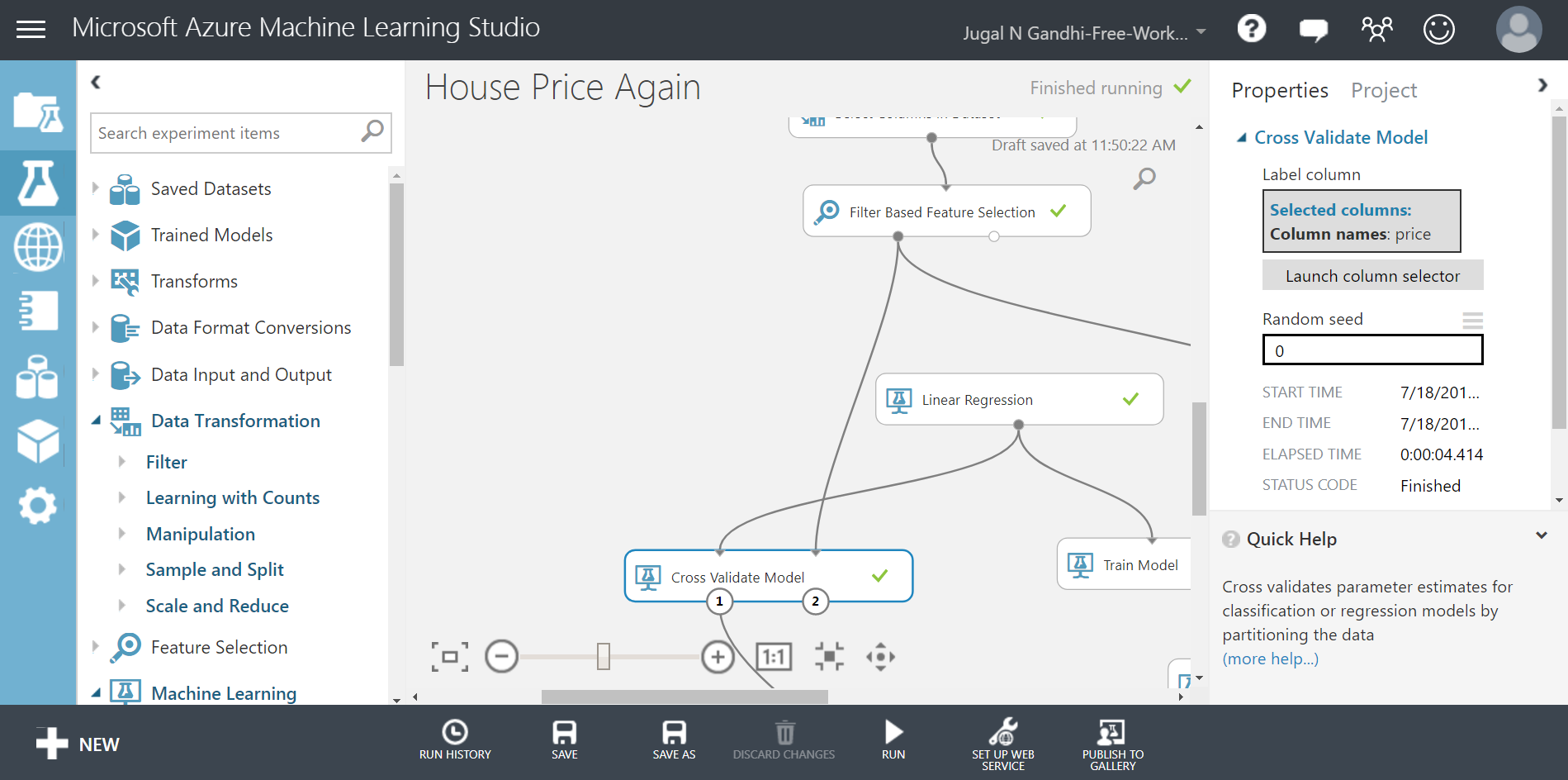
As seen from the above image, one input to this Cross-Validate Model module will be Linear Regression module which is the type of machine learning model we want to train and other input will be Filter Based Feature Selection module which the entire dataset that we want the model to learn.
Evaluating the results
In this exercise we shall learn how to evaluate the machine learning model’s results.
-
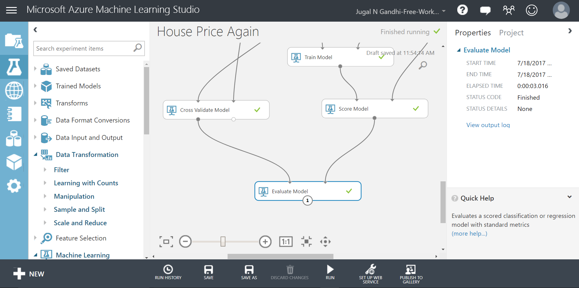
STEP 1: Select Machine Learning->Evaluate from the left panel and drag the Evaluate Model module in you experiment canvas.
-
STEP 2: Select the Evaluate Model module and click to visualize the evaluation results.
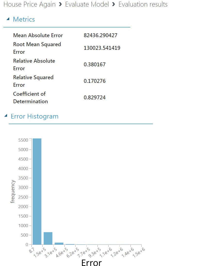
As shown above, our linear regression model has a R-square(Coefficent of Determination) value of 0.83. This means 83% of variation in price values can be described by the variation in the values of feature columns(predictors). This is really a high value in context of house price prediction problems. Depending on problem optimal value of R-square changes. For house price prediction problem, any R-square value above 0.75 is really good.
To understand the meaning of the other metrics, visit here.
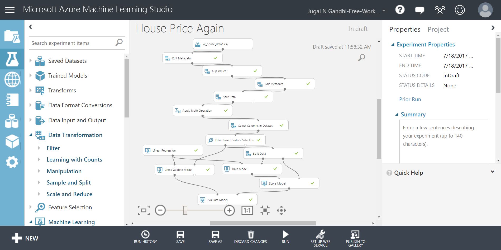
The final picture of our experiment canvas should be like below: